Как сделать to do list в excel?
Содержание
- 1 Excel To Do List Templates (Free Download)
- 2 Steps to Creating a To Do List in Excel
- 3 Adding check boxes in your to-do list
- 4 To Do List Templates (Excel)
- 5 Conclusion
- 6 1. Simple Drop-Down Lists via Data Validation
- 7 2. Conditional Formats for the Priority Column
- 8 3. Conditional Formats for Numeric Priority
- 9 4. Checkboxes using Form Fields
- 10 5. Checkboxes via Data Validation
- 11 6. Progress Bar for % Completed
- 12 7. Gray-Out Tasks When They are Complete
- 13 8. Highlighting Overdue Dates
- 14 9. Autofilter and Sorting
- 15 10. Create a Gantt Chart
- 16 11. Drop-Down with Current Date
- 17 Ссылки
You start your day. Plan some tasks. Write it down somewhere and start working on it.
When it’s way past your work time, you think about that to-do list (stare at it if you have it written) and curse the world for not having enough time in the day.
Sounds familiar?
If you are nodding your heading in agreement, you – my friend, are suffering from an acute condition of expanding-to-do-list.
Well, I am neither a brain doctor nor a self-help guru. I can not help you in overcoming procrastination and getting your work done.
BUT…
I can give you an Excel To Do List template that can handle your ever-expanding list (you will still have to make one and do all the work).
Jokes aside, I do believe it is helpful when you maintain a to-do list. I create one every morning, and on some lucky days, I also get the pleasure of checking off most (if not all) the items.
Excel To Do List Templates (Free Download)
Here are the four Excel To Do List templates you can download:
- A Simple printable Excel To-do List.
- To-do List with drop downs to mark a task as complete.
- To-do List where you can check a box to mark a task as complete.
- To-do List where you can simply double to mark the task as complete.
Excel To Do List Template #1 – Printable To Do List
This one is for people like me.
I like to print my to-do list and stick it right in front of my eyes and then work on the items on the list.
Here is a simple Excel template where you can fill the tasks and take a print-out. If you prefer writing the tasks yourselves, simply print it first and then fill in the tasks.
There is a separate column to mention date and comments (if any). If you don’t need it, delete these columns before printing.
Download simple printable to-do list template
Excel To Do List Template #2 – With Drop Down List
If you prefer making and maintaining the To Do list in Excel itself, you are in for a treat.
Here is an Excel To Do List template where you can:
Additional Notes:
- The weights are given as follows (in the pic below). If you want to change the weights, you can easily do it by changing these values. In the download file, columns G to J are hidden. Unhide it to change the weights.
- To calculate progress using the progress bar, we calculate:
- Total Score: Add all the weights for all the activities. For example, if there are 2 high priority tasks and 1 medium priority task, and 1 low priority task, the total score would be 14 (5+5+3+1).
- Completed Score: Here we add all the weights for all the activities that are completed. For example, if out of 4 activities, 1 high priority activity has been completed, then the Completed Score would be 5.
- % Completed: The value when we divide Completed Score with Total Score. For example, in the above case, it would be 35.7% (5/14).

Download to-do list with drop-downs
Excel To Do List Template #3 – With Check Boxes
This template is exactly like the one with drop downs, with a minor difference – it has checkboxes instead of the drop-down.
You can mark the task as complete by checking the checkbox. If not checked, it is considered incomplete.
Here is how you can use this Excel To Do List Template:
NOTE: Be careful while adding deleting rows. Deleting a row does not delete the checkbox.
— Регулярная проверка качества ссылок по более чем 100 показателям и ежедневный пересчет показателей качества проекта.
— Все известные форматы ссылок: арендные ссылки, вечные ссылки, публикации (упоминания, мнения, отзывы, статьи, пресс-релизы).
— SeoHammer покажет, где рост или падение, а также запросы, на которые нужно обратить внимание.
SeoHammer еще предоставляет технологию Буст, она ускоряет продвижение в десятки раз, а первые результаты появляются уже в течение первых 7 дней. Зарегистрироваться и Начать продвижение
Download to-do list template with checkboxes
Excel To Do List Template #4 – Double-click Enabled
I find this version of the template the best of all.
It uses a small VBA code to enable the double click event where you can mark a task as completed by simply double-clicking on it.
NOTE: Since this contains a VBA code, it should be saved in .XLS or .XLSM format.
Here is how you can use this Excel To-do List Template:
Download Excel Template To Do List #4 – Double Click Enabled
NOTE: Since this template contains a VBA code, when you open it, Excel will show a prompt to enable content. You need to enable it for this to work.
![]()
So here are 4 Excel To-do list templates that I find useful and often use while planning my work.


Common Use Cases of Using these To-do list templates
While I have shown you the example of common daily tasks, you can use these to-do list templates in many different ways.
Here are some use cases that come to my mind:
- Project Management Checklist: Since a project can have many moving parts to it, creating a daily or even weekly/monthly to-do lists can help you keep a tab on all the important stuff.
- Client onboarding checklist: You can create a quick client onboarding checklist and hand it over to your sales/customer executives. This will make sure a client gets seamless and complete onboarding experience.
- Grocery checklist: While it may sound weird to create one in Excel, I have seen people do this. This has become more useful now that we can order stuff groceries online in a few minutes.
- Event Management Checklist: Event management can get crazy and out of control if not planned well. A handy to-do list can save you (and others) a lot of time and money.
- Travel Itinerary and Packing checklist: I love to keep my traveling hassle-free by having a to-do list of stuff that needs to be done (bookings, visa, tickets, etc). You can also create a packing list to make sure you don’t leave important stuff behind.
- Blog Publishing Checklist: I have created a to-do list to make sure I don’t miss out on the important parts when publishing a blog post on this site. These tasks include doing grammar and spell-check, making sure titles are correct, images are present, tahs and categories are assigned, etc.
What goes into making the Excel TO DO List template?
There is no rocket science at play here. Simple Excel techniques come together to make it happen.
Here are the components that make these templates:
- Conditional formatting (to highlight a row in green when a task is marked as completed).
- Strikethrough Format (appears when a task is marked as completed).
- Excel Drop-down Lists (to show the status in the drop-down).
- Check Boxes (to mark a task as complete by checking it).
- VBA (to enable double click event).
- Excel Charting (to create the progress bar).
I hope these templates will help you become more productive and save some time.
I am sure you also have tons of To-do list success/failure stories and I would love to hear it. I am waiting in the comment section 🙂
Other Excel Templates You Might Like:
- To Do List template Integrated with Calendar in Excel.
- Task Prioritization Matrix Template in Excel.
- Shared Expense Calculator in Excel.
- Employee Timesheet Calculator.
- Vacation Itinerary and Packing List Template.
A to-do list is very important in ensuring that you conduct all of your important daily activities. One of the character traits of humans is being forgetful, so sometimes you can come to the end of the day only to realize that you forgot a certain task. A to-do list does away with all the possibilities of forgetting something that you wanted to do. Examples of to-do lists that you can have include shopping, work, assignments and targets to meet. Luckily, you can create your own to do list using Excel from your computer. This article shows you how you can create a to-do list with checkboxes using excel.
Steps to Creating a To Do List in Excel
To create your To Do list effectively, follow the steps below:
- Depending on the to do list that you want to create, open Excel application and add relevant column headers. These may include tasks, priority, status, due date and done/completed.
- After creating the column headers, fill them with relevant information. This includes all the tasks that you want to accomplish in order of their relevance.
- At the Home tab, highlight the column headers then click on the center icon to center the highlighted text.

Adding check boxes in your to-do list
Your to-do list is more fun and easier to accomplish if you add check boxes. These will remind you of the tasks that you have not accomplished easily. Here is how to add check boxes to your to-do list:
- Click on File> options then select the customize ribbon located in the pop-up box.
- Looking at the right side where the Main Tabs are located, you will see a box next to Developer. Click on it, and you should see a new developer tab added to your excel file.

- On the Developer tab, click insert and select the checkbox option.
 4. Click on the area where you want your checkbox to appear, and it will automatically do so.

- To enable editing, right click on the text. You can use the provided text or delete them and add yours. You can also resize the boxes at this stage.
- After putting your checkbox in a cell, click on it and drag down to the other columns so that you can auto-populate the checkboxes.
- Create a formula that will help you determine whether the information put on the check boxes is true or false.
To Do List Templates (Excel)

Download
Task To Do List Template

Download
To Do List with Due Date (Excel)

Download
Priority To Do List Template (Excel)

Download

Download

Download
Conclusion
To do lists are very important in helping to work on all of your day’s tasks. Fortunately, you can create one using excel as shown above depending on what you want to achieve.
— Разгрузит мастера, специалиста или компанию;
— Позволит гибко управлять расписанием и загрузкой;
— Разошлет оповещения о новых услугах или акциях;
— Позволит принять оплату на карту/кошелек/счет;
— Позволит записываться на групповые и персональные посещения;
— Поможет получить от клиента отзывы о визите к вам;
— Включает в себя сервис чаевых.
Для новых пользователей первый месяц бесплатно. Зарегистрироваться в сервисе
One of the best ways to learn new techniques in Excel is to see them in action. This post demonstrates how to add some fun and useful features to simple to do lists including drop-down lists, check boxes, progress bars, and more. The images show Excel 2016, but instructions are similar for Excel 2010 and Excel 2013.
1. Simple Drop-Down Lists via Data Validation
Many task lists include a Priority or Status column, such as the Homework To Do List shown below. It’s very handy to use an Excel drop down list for columns like these.

To create a simple drop-down list, follow these steps:
- Select the cells you want to edit
- Go to Data > Data Validation
- Choose «List» in the Allow field
- In the Source field enter a comma-delimited list such as High,Medium,Low
2. Conditional Formats for the Priority Column
In the example above you will see that the values in the Priority column have been highlighted differently. This can be done automatically and is a great way to easily identify your high-priority tasks. Follow these steps to create the type of formats shown in the example above.
- Select the cells in the Priority column
- Go to Home > Conditional Formatting > Text That Contains
- Enter the word high and choose the «Light Red Fill with Dark Red Text» option
The image below shows how to get to the correct option from the Home tab.

3. Conditional Formats for Numeric Priority
If you want to use a numeric priority like 0-4, then you can use Icon Sets to display images instead of (or in addition to) the numeric value. You can see this demonstrated in the Simple Task Tracker below.
- Select the cells in the Priority column
- Create a drop-down list with the options 4,3,2,1
- Go to Home > Conditional Formatting > Icon Sets > More Rules
- The image below shows you how to modify the settings for this rule.
4. Checkboxes using Form Fields
I don’t like this method. If you like to sort and delete and insert rows, form fields get all messed up. They may be nice for a spreadsheet layout that is not meant to be modified, but so far I haven’t found a to do list that I haven’t wanted to modify frequently.
The form field checkbox is found in the Developer tab shown in the image below. If you don’t see the Developer tab, go to File > Excel Options > Customize Ribbon and find and check the Developer tab.
5. Checkboxes via Data Validation
I wish Microsoft would add an in-cell checkbox feature (Apple’s Numbers software does it), but until they do that we have to come up with clever alternatives.
One method I like is using a data validation drop-down list because it works pretty well in Excel on touch-enabled devices, and it is also compatible with most versions of Excel and OpenOffice and Google Sheets.
The simplest checkbox to make using a drop-down list is probably just a list with a single character (x), or you could use a special character like the square root sign (√) that looks like a check mark in some fonts. In the example below, I’ve used this technique plus a small square ascii character (□,√).
Another approach that I really like is to use custom Icon Sets via Conditional Formatting. This isn’t as compatible with other spreadsheet programs (like Google Sheets) but it looks good. The simple Task Tracker Template shows an example of this:
- Select the cells you want to use for the check boxes
- Create a drop-down list with the options 1,0,-1
- Go to Home > Conditional Formatting > Icon Sets and select any set you like
- With those cells still selected, go to Home > Conditional Formatting > Manage Rules and find the rule you just created and edit it to create a custom icon set with the setting shown in the following image.
Another example that uses this technique is my Financial Plan Summary template.
6. Progress Bar for % Completed
In some of the examples above, you’ve already seen progress bars in the «% Complete» column. Now you’ll learn how to do it. Conditional formatting comes in handy yet again:
- Select the cells in the % Complete column
- Go to Home > Conditional Formatting > Data Bars > More Rules
- Modify the bar based on the settings shown in the image below
What a Progress Bar in Google Sheets? No problem. In cell A1 enter the % Complete and then in the cell to the right of it you can use the formula =REPT(«█»,ROUND(A1*10,0)). You can change the color of the bar by just changing the font color. That’s a pretty old trick for Excel users, but it’s something that will work in Google Sheets, too.
7. Gray-Out Tasks When They are Complete
If you like the effect of seeing your completed tasks crossed out or grayed out or both, you can do that fairly easily using conditional formatting.
In the example below, the first rule is applied when column A is equal to the special square root character. The placement of the dollar sign in the $A4 reference is very important in this formula because we want all the columns in the table to reference column A.
Also note that the first rule has the «Stop if True» box checked. That is why you don’t see the priority cell highlighted red or the % Complete showing a green bar in the example. When the task is marked as complete, I don’t want to be distracted by formatting that no longer matters to me. So I’m using the rule order to prevent the following rules from being applied if the task has been marked as done.
8. Highlighting Overdue Dates
When you have a Due Date, you may want to highlight the date when it is overdue. You can do that with a simple conditional formatting rule shown in the example below.
You can see an example of this in the Homework To Do List shown at the very top of this article.
9. Autofilter and Sorting
The little arrows that show up in the header of an Excel table or list are a result of turning on the Filter Button feature. If you don’t see the little arrows in the header row already, select a cell in your table (or the entire table) and go to the Data tab and click on the Filter button.
10. Create a Gantt Chart
Although a Gantt chart is a great visualization and management tool for projects, creating one from scratch is not nearly as simple as the other ideas shared in this article. The two most common ways to create a Gantt chart in Excel are (1) using a stacked bar graph chart object and (2) using conditional formatting. Visit my Task List Templates page to find an example that uses a chart object and try the free Gantt Chart Template to see the conditional formatting technique in action.
11. Drop-Down with Current Date
Update 10/9/2018 — I recently created a new wedding checklist where a user requested the ability to enter either a checkmark or the current date. To do this with data validation, create a list somewhere in the worksheet with the first cell containing a check mark unicode character ✔ and the next cell containing the formula =TODAY().
Then, use data validation to create a drop-down list referencing those two cells. This will allow you to select either a checkmark or the current date as shown in the image below.
To avoid having Excel show warnings when cells contain older dates, make sure to turn off the warnings and errors when setting up the data validation.
Небольшое Excel-приложение, эмулирующее простой To-Do-лист сделанную в духе матрицы Эйзенхауэра.
Позволяет наглядно отслеживать задачи — что нужно сделать, что делается и что сделано.)
Задачи, в зависимости от статуса реализации, записывается в ячейку нужной цветовой зоны. Задачи можно переносить из одной зоны в другую — для этого просто нужно навести курсор на границу ячейки и перетащить, зажав левую кнопку мыши.
Чтобы вообще удалить задачу, нужно просто выделить ячейку с ней и нажать на клавиатуре Delete. При добавлении/удалении, а также изменении статуса задач окрашивание ячеек происходит автоматически. Собственно, тут и понадобились макросы. 🙂
Тип данных во всех ячейках на листе — многострочный текст. Используйте комбинацию Alt + Enter, чтобы создавать заметки из двух-трёх строк.
Рабочая область разделена на 4 зоны:
- Зелёная — важно и несрочно — планируемые важные задачи. Самый главный квадрант. Спокойное планомерное выполнение задач из этой области ведёт к достижению целей.
- Жёлтая — важно и срочно — текущие задачи, которые необходимо выполнить прямо сейчас. Необходимо всячески стремиться, чтобы этот квадрант был пустым, т.е. откладывать все второстепенные дела и выполнять важносрочные задачи.
- Серая — неважно, срочно — Небольшие задачи, возникающие в течении дня и способствующие решению важных задач из жёлтой или зелёной области.
- Чёрная — неважно, несрочно — несущественные несложные дела, которыми мы занимаемся лишь бы не выполнять задачи из других квадрантов.
В основной области автоматически выделяется красная подобласть. Её размер зависит от жёлтой зоны.
Следует обратить внимание на эту область. Она логически определяет центр и влияет на раксраску квадрантов. Значение ячееек этой области нельзя менять (по тексту всех 4-х ячеек макрос идентифицирует логический центр, если текст изменить, то идентификация станет невозможной).
Однако при этом разрешается перенести центр. Для этого необходимо выделить одновременно все 4 ячейки, навести курсор на границу ячеек и перетащить эту группу ячеек в другое место. В соответствии с новым расположением изменится расцветка квадрантов, которые изменятся в размерах.
Ссылки
Скачать excel-приложение «To-Do» с Гугл-Диска
Musadya
|
November 5, 2011
|
Other
|
There are several to do list templates that you can find as part of my excel templates. For example in my daily planner template and gantt chart template. But, if you need a more simple and standalone to do list template, you can use this one. I called it simple because there is no time or date references inside this template. There are only task name and completion status that you have to fill. It is will be more suitable for kind of jobs or tasks that have to be finished without any strict completion time or date or to be finished within one day or short period of time.
There are two kind of templates available. The first one is a single to-do list where it is more suitable to be used for single person. Inside it, there are 26 rows that you can use to fill your tasks. There are no excel formula inside the table. Just type the number, type your tasks name, and type a completion status once you finished your tasks. You can put word “done” or type “v” or any other characters. Remember to leave the status column blank when the tasks are not finished yet. The reason why you have to leave it blank, because the completion bar on top of the table will calculate the percentage of finished job by counting the number of columns that is not blank. You can modify this excel formula to suit your needs.
The second one is the team to do list. Basically, it is an aggregation of single to-do list templates with additional summary where you can see accomplishment of any members in this team. For example, it can be used to monitor the performance for any voluntaries project that is held in one day. Or, it can be used to measure performance of its member for doing the same job within the same period of time. To use this template is the same with the first template, except you can switch between to-do list from summary worksheet by selecting it from the column name. You can download both templates below which is only can be opened if you are using Microsoft Excel 2007 or 2010.
To Do List V1.0 (12.2 KiB, 9,649 hits)
Team To Do List V1.0 (61.0 KiB, 6,970 hits)